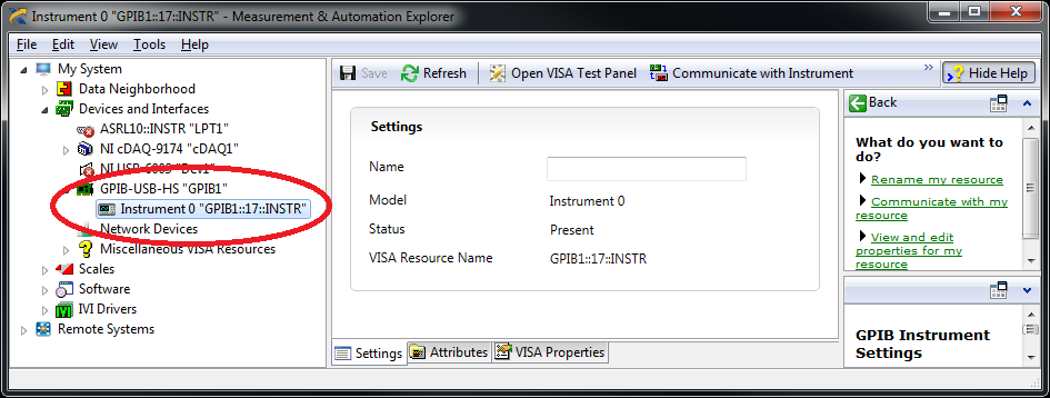
Finding the instrument and card index using NI MAX
This software provides remote operation, data acquisition, and data processing capabilities for the HP 4192A impedance analyzer.
This software is provided as a win32 binary, and should be capable of running on most PCs running Windows XP through Windows 10. Source code and binaries for other platforms are not available. Additional requirements include:
Users will benefit from reading the HP 4192A product manual prior to using the instrument.
Install LabVIEW RE and 488.2 software packages prior to using this software. Then connect the GPIB adapter, power on the impedance analyzer, and take note of the GPIB address displayed on the unit during start-up. The default address is 17; see manual section 3-117.
Upon launching the software, if everything is configured correctly, measurements will begin immediately. Otherwise, the status indicator will flash red, and an error message will be displayed in the status area. The following troubleshooting steps are suggested if this occurs:
When running, the software continuously triggers the 4192A instrument to perform measurements, unless "Pause reading" is selected.
Instrument control settings are immediately sent to the instrument.
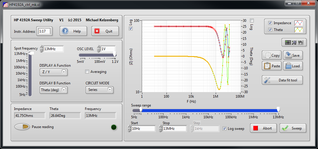
Frequency sweeps can be specified using the sweep range sliders, or by entering values directly into the "start" and "stop" fields.
Selecting Log sweep will use logarithmically spaced frequency values for the sweep, and will change the display graph's X-axis to logarithmic mapping. In this mode, the spacing of data points is determined by the 4192A instrument, and cannot be changed in software.
Once a sweep is started, either within the software or using the instrument's front panel buttons, data will be collected and displayed in the graph area. The sweep can be aborted or paused in software. Generally, attempting to use the instrument's front panel buttons during a sweep will interfere with data collection, and may lead to the graph data being erased.
Note: Using "AUTO" circuit mode may have undesired effects during frequency sweeps. If the instrument automatically changes circuit modes during a sweep (e.g., series to parallel), the subsequent measurements are of a different type than the existing measurements (e.g., admittance vs. impedance) and cannot be plotted on the same graph axes. The software, recognizing the change in measurement type, will clear the existing data from memory, effectively truncating the sweep range. It is thus recommended to avoid "AUTO" circuit mode for sweeps.
After (or during) a sweep, the collected data can be saved to a text file, or copied to the clipboard. The file format is tab-separated ASCII. Copied data can be pasted directly into most spreadsheet programs such as Excel.
Prior sweep data can be loaded (or pasted) to enable graphing or analysis of the measurements. The imported data must be of the same format as that which is saved (or copied) from the program. When loading prior data, a dialog box will appear to enable selection of the measurement type.
The data fit tool is useful for making sense of frequency sweep measurements. Unlike single-point measurements of capacitance or inductance, frequency sweeps generally reveal varying impedance trends due to, for example, self-resonance effects, transmission lines, or the combination of multiple circuit elements. Fitting the sweep data to a circuit model can reveal the effective topology of a complex circuit, or produce an accurate equivalent model of a component or subcircuit for use with computer simulation.
To produce the data shown the example screenshot shown below, I connected a capacitor and inductor of unknown value, in parallel, at the far end of an unknown length of RG223 cable. A frequency sweep was performed from 10 Hz to 13 MHz. By selecting an appropriate equivalent circuit model, and adjusting parameter values to obtain good fit agreement, the unknown values for capacitance, inductance, and line length can be calculated with reasonable accuracy.
Although this example illustrates several unknowns being resolved by a single swept impedance measurement, it should be noted that the greatest accuracy occurs when each circuit element is analyzed independently, if possible.

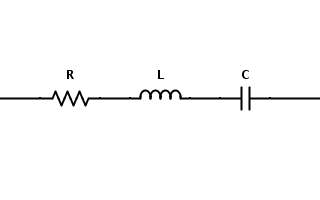
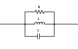
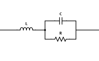
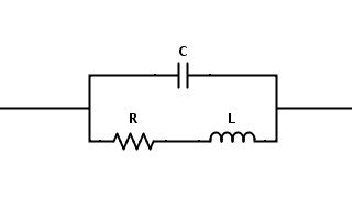
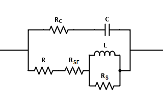
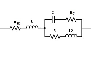
Each circuit model includes a number of elements, namely: resistors, capacitors, inductors, and an optional transmission line. The selected model's schematic is shown above the parameter value table. As the values of each parameter are changed, the corresponding impedance data is plotted against the measurement data. The objective is to select the circuit model best approximating the measured impedance, and then to adjust the parameter values to obtain optimal agreement between model and measurement data.
If certain parameters' values are known, you should enter them directly (e.g., transmission line impedance). The easiest way to "tune" the remaining parameters' values is using the mouse wheel. Position the cursor over the value entry box, then scroll the wheel up or down to adjust. The following modifier keys can be used:
Depending on the model chosen, it makes sense to tune certain parameters (e.g., parasitic resistors) to their max/min values before attempting to tune for the more interesting parameters.
The software can sometimes automatically determine parameter values for an optimal fit. This approach relies on simplex optimization, and is generally only useful when presented with a good starting guess. However, once approximate values for each parameter are established, this feature will quickly and easily finalize the fit.
To attempt auto-fitting of the data, select the appropriate circuit model and coarse-tune the fit parameters to reasonable values. This is especially important for parameters that tend to dominate the model behavior at default values. For example, make sure that shunt resistances are set to a high value.
Then, specify the criteria for the fit. All impedance measurements produce two real data sets which uniquely describe a complex impedance value, for example, impedance magnitude Z and phase theta. These data sets are plotted in the two graphs to the left. Next to each is a fit criteria ("optimize type") drop-down menu. You may select any of the three self-explanatory fit criteria for one or both data sets. At least one data set must have an active fit criteria selected, and generally, fitting both sets simultaneously is appropriate.
Additional fit options are shown to the upper right. These include a relative fit tolerance (suggested value: 1E-4 to 1E-10) and an iteration limit for the fit process (suggested value: 10k or higher). A smaller tolerance value, or larger iteration limit, might produce a better fit. However, to prevent software lock-up, there is a hard-coded time limit for each fit attempt. Requesting excessively tight fit tolerance will thus cause the fit to time out. For curiosity, you can also select to "show fit progress," which will update the graphs at each iteration (guess) of the fitting process. This slows down the fitting process considerably, and may cause the fit to time out.
Pressing the "fit" button will attempt to tune all active parameter values, to optimize the model fit to experimental data. Sometimes the attempt will fail to improve the model fit, or even make it worse. If this happens, previous values can be restored with the "undo" button.
It is not possible to lock or constrain individual parameters. If certain values need to be fixed, it may be necessary to manually reset these parameters (if changed) after optimization, then manually tune the remaining free parameters until reasonable fit is restored. Sometimes it is of use to repeat the fit after manual adjustment, as the outcome of the fit might be different given a new starting guess.
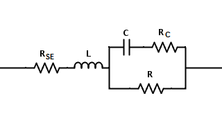
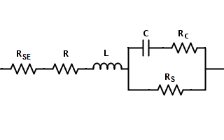
The following circuit models are available.
 |
 |
 |
 |
 |
 |
 |
 |
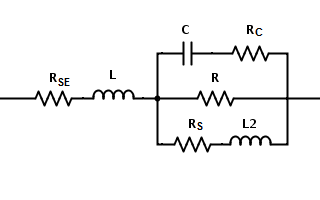 |
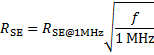
Skin effect causes the effective resistance of conductors to increase with frequency. The actual resistance vs. frequency behavior due to skin effect is complex, and depends strongly on the specific geometry and composition of the circuit elements. However, for typical (e.g. cylindrical) conductors, above a certain frequency, the conductor resistance tends to increase as the square root of frequency. To provide a crude means of modeling the skin effect resistance increase at high frequencies, some of the circuit models included with this software include a "skin effect resistor," RSE. The value of this resistance is calculated as:
It is sometimes inconvenient or impossible to locate the circuit to be tested directly at the 4192A's test fixture terminals. In these cases, a length of transmission line can be used between the instrument and the unknown circuit. The data fit software utility makes it easy to account for the effect of this feedline when analyzing the data.
I frequently use a length of RG223 or similar coaxial line, adapted at the near end directly to the 16047A test fixture. The outer conductor should be connected to the "Low" terminal.
For optimal accuracy, the selected feedline should first be characterized over the frequency range of interest, using a well-known load at its far end -- for example, terminating a 50-ohm line with a precision 75-ohm resistor. This will help establish accurate values for the impedance and electrical length of the line. Measuring the length and velocity of the line will also help.
As any victim of E/M coursework knows, the greatest virtue of the transmission line is its frequency-independent characteristic impedance:

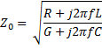
Where for the discussion here, L, C, R, and G are the transmission line's distributed (or, per-unit-length) inductance, capacitance, resistance, and conductance. This leads to Smith charts; then somehow to profit, right? But an afternoon on your therapist's couch might help you recover this long-repressed memory: that finite conductance and dielectric leakage conspire to give a frequency-dependent equation for characteristic impedance:
With normal (good) conductors and normal (high) frequencies of interest to the RF engineer, the R and G terms can be safely neglected to yield the familiar equation:

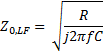
However, at especially low frequencies, the dissipative terms come into play--or at least one of them. It turns out that for typical transmission line geometries, at low voltages, the dielectric leakage remains incredibly small, so we may continue neglecting G. However even the best conductors (that you can afford, at least) have enough resistance to affect Z0 at lower frequencies. This gives us:
Let us define a frequency fT at which |Z0,LF| = Z0,HF. We find that:
We can now re-arrange the frequency-dependent equation for Z0, still assuming G = 0, as:
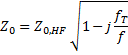
This provides a convenient expression for the transmission line's characteristic impedance, which I believe to be approximately valid from the lower range of useful frequencies for impedance analysis, through the higher frequencies (up to the onset of skin-effect behavior). Also, we need only a single parameter fT to model this behavior with our circuit calculator, which can be determined empirically or by calculation based on known properties of the line. A quick internet search for properties of RG58 cabling suggests that the value of fT for this line should be around 20 kHz.
It should be noted that the above considerations are at best a first-order approximation; there are numerous other factors that lead to frequency-dependent characteristic impedance of a transmission line. A particularly instructive discussion can be found here.
In practice I have not encountered situations where modeling the low-frequency impedance of a transmission line has been particularly important in the analysis of impedance sweeps. Moderate effects can be observed when measuring long lengths (10+ meters) of low-conductivity coax. To effectively disable this model, set the value of fT to a low frequency such as 1 Hz.
The 4192A instrument is capable of performing voltage (bias) sweeps with DC bias ranging from (up to) +/- 35 V. This is useful, for example, for studying the C-V behavior of a semiconductor p-n junction.
This software does not directly support voltage sweeps; however, it can be used to collect (and save) the data from a voltage sweep using the following procedure. In the following narrative, I'll perform a C-V sweep on a commercial TVS diode and extract the parameters Cj0, VBI, and m, which I could then use in creating a SPICE model for the diode.
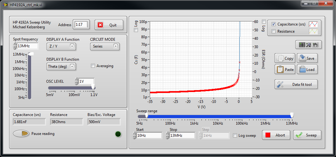
Upon resuming measurements, the software will recognize that a voltage/bias sweep is underway. The graph X-axis will be updated to show bias value instead of frequency. After the completion of the sweep, you may save or otherwise export the data for analysis. The screenshot above shows the data acquired when measuring a commercial TVS diode. A simple Excel spreadsheet can be used to extract Cj0, VBI and m; in this example:
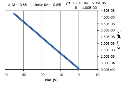 Diode fit from example Excel spreadsheet |
Extracted parameters | |
| Cj0 = 30 pF | ||
| VBI = 0.49 V | ||
| m = 0.35 | ||
The following additional considerations should be observed when performing bias sweeps:
This software is freeware, for non-commercial use only. For commercial use, please contact me.
You may use this software for free, for non-commercial purposes only, on as many computers as you want, for as long as you see fit; however, you may not sell this software, include it in a product, or offer it for download on your web site. The complete license is included with the software.
If you find this software to be especially useful, please write me a note to let me know, or acknowledge it in your paper or thesis. Alternately, you may mail me one million dollars in small, unmarked bills. Your support will be greatly appreciated.
Michael Kelzenberg

This software is provided for free. Technical support is not generally available; however, feel free to contact me with bug reports or ideas.
 Download this example sheet